I might use neural autoregressive distribution estimators (NADEs) for the speech synthesis project; this has to do with an idea both Guillaume Desjardins and Yoshua Bengio talked about in the past couple days, and which I’ll detail later on. For now, I’d like to test my understanding of NADEs by introducing them in a blog post. As they say,

If you want to learn something, read. If you want to understand something, write. If you want to master something, teach.

The idea

RBMs are able to model complex distributions and work very well as generative models, but they’re not well suited for density estimation because they present an intractable partition function: \[ p_{RBM}(\mathbf{v}) = \sum_{\mathbf{h}} p(\mathbf{v}, \mathbf{h}) = \sum_{\mathbf{h}} \frac{ \exp(-E(\mathbf{v}, \mathbf{h})) }{ \sum_{\tilde{\mathbf{v}}, \tilde{\mathbf{h}}} \exp(-E(\tilde{\mathbf{v}}, \tilde{\mathbf{h}})) } = \sum_{\mathbf{h}} \frac{\exp(-E(\mathbf{v}, \mathbf{h}))}{Z} \] We see that \(Z\) is intractable because it contains a number of terms that’s exponential in the dimensionality of \(\mathbf{v}\) and \(\mathbf{h}\).

NADE (original paper) is a model proposed by Hugo Larochelle and Iain Murray as a way to circumvent this difficulty by decomposing the joint distribution \(p(\mathbf{v})\) into tractable conditional distributions. It is inspired by an attempt to convert an RBM into a Bayesian network.

The joint probability distribution \(p(\mathbf{v})\) over observed variables is expressed as \[ p(\mathbf{v}) = \prod_{i=1}^D p(v_i \mid \mathbf{v}_{<i}) \] where \[ \begin{split} p(v_i \mid \mathbf{v}_{<i}) &= \text{sigm}(b_i + \mathbf{V}_{i}\cdot\mathbf{h}_i), \\
\mathbf{h}_i &= \text{sigm}(\mathbf{c} + \mathbf{W}_{<i}\cdot\mathbf{v}_{<i}) \end{split} \]

As you can see both in the graph and in the joint probability, given a specific ordering, each observed variable only depends on prior variables in the ordering. By abusing notation a little, we can consider \(\mathbf{h}_i\) to be a random vector whose conditional distribution is \( p(\mathbf{h}_i \mid \mathbf{v}_{<i}) = \delta(\text{sigm}(\mathbf{c} + \mathbf{W}_{<i}\cdot\mathbf{v}_{<i})) \).

The distribution modeled by NADEs has the great advantage to be tractable, since all of its conditional probability distributions are themselves tractable. This means contrary to an RBM, performance can be directly measured via the negative log-likelihood (NLL) of the dataset.

In (Larochelle & Murray, 2011), NADEs are shown to outperform common models with tractable distributions and to have a performance comparable to large intractable RBMs.

Implementation and results

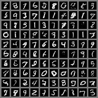
I ported Jörg Bornschein’s NADE Theano implementation to Pylearn2 and used it to reproduce Larochelle & Murray’s results on MNIST. I intend on making a pull request out of it so it’s integrated in Pylearn2.

The trained model scores a -85.8 test log-likelihood, which is slightly better than what is reported in the paper. To be fair, I made a mistake while training and binarized training examples every time they were presented by sampling from a Bernoulli distribution, which explains the better results.

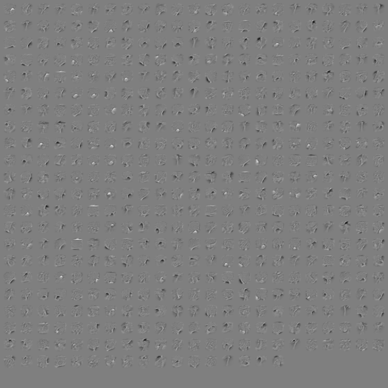
Below are samples taken from the trained model (more precisely parameters of the Bernoulli distributions that were output before the actual pixels were sampled) and weights filters.