This semester I’m taking Yoshua Bengio’s representation learning class (IFT6266). In addition to formal evaluation, we’re also evaluated in the context of a big class project, in which we compete against each other to find the best solution to a machine learning problem. We’re to maintain a blog detailing our progress, and we can cite or be cited by other students, in analogy to what’s done in actual research.

Suppose you have a good, real-valued representation of audio frames and you wish to learn the distribution of the next audio frame conditioned on the previous one. The following DBM can achieve that:

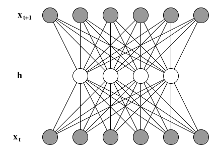
It is a three-layered DBM whose first and last layers are gaussian and whose hidden layer is binary.

Let’s start with the energy function:

\[ E(\mathbf{x}^t, \mathbf{h}, \mathbf{x}^{t+1}) = E_{bias}(\mathbf{x}^t, \mathbf{h}, \mathbf{x}^{t+1}) + E_{interact}(\mathbf{x}^t, \mathbf{h}, \mathbf{x}^{t+1}) \]

with

\[ E_{bias}(\mathbf{x}^t, \mathbf{h}, \mathbf{x}^{t+1}) = \frac{1}{2}(\mathbf{x}^t - \mathbf{b})^T(\mathbf{x}^t - \mathbf{b})

• \mathbf{c}^T\mathbf{h}
• \frac{1}{2}(\mathbf{x}^{t+1} - \mathbf{d})^T(\mathbf{x}^{t+1} - \mathbf{d}) \]

and

\[ E_{interact}(\mathbf{x}^t, \mathbf{h}, \mathbf{x}^{t+1}) =

• \mathbf{h}^T\mathbf{W}\mathbf{x}^t
• (\mathbf{x}^{t+1})^T\mathbf{U}\mathbf{h} \]

Sparing you the algebraic details, conditional probabilities for this model are given by

\[ \begin{split} p(\mathbf{x}^t \mid \mathbf{h}, \mathbf{x^{t+1}}) &= \mathcal{N}(\mathbf{x}^t \mid \mathbf{b} + \mathbf{W}^T\mathbf{h}, \mathbf{I}), \\
p(\mathbf{h} \mid \mathbf{x}^t, \mathbf{x^{t+1}}) &= \text{sigmoid}(\mathbf{c} + \mathbf{W}\mathbf{x}^t + \mathbf{U}^T\mathbf{x}^{t+1}), \\
p(\mathbf{x^{t+1}} \mid \mathbf{x}^t, \mathbf{h}) &= \mathcal{N}(\mathbf{x}^{t+1} \mid \mathbf{d} + \mathbf{U}\mathbf{h}, \mathbf{I}) \end{split} \]

and the gradient of the negative log-likelihood (NLL) of \(p(\mathbf{x}^{t+1} \mid \mathbf{x}^t)\) is given by

\[ \begin{split} \frac{\partial}{\partial \theta} -\log p(\mathbf{x}^t \mid \mathbf{x^{t+1}}) = &\mathbb{E}_{p(\mathbf{h} \mid \mathbf{x}^t, \mathbf{x}^{t+1})} \left[ \frac{\partial}{\partial \theta} E(\mathbf{x}^t, \mathbf{h}, \mathbf{x}^{t+1}) \right] \\\ - &\mathbb{E}_{p(\mathbf{h}, \mathbf{x}^{t+1} \mid \mathbf{x}^t)} \left[ \frac{\partial}{\partial \theta} E(\mathbf{x}^t, \mathbf{h}, \mathbf{x}^{t+1}) \right] \end{split} \]

For the positive phase, you sample from \(\mathbf{h}\) given \( \mathbf{x}_t \) and \( \mathbf{x}_{t+1} \) and for the negative phase, you sample from \( \mathbf{h} \) and \( \mathbf{x}_{t+1} \) given \( \mathbf{x}_t \).